Optimizers

• Momentum and Nestorov’s method improve convergence by normalizing the mean (first moment) of the derivatives
• Considering the second moments
  • RMS Prop / Adagrad / AdaDelta / ADAM¹
• Simple gradient and momentum methods still demonstrate oscillatory behavior in some directions²
  • Depends on magic step size parameters (learning rate)
• Need to dampen step size in directions with high motion
  • Second order term (use variation to smooth it)
  • Scale down updates with large mean squared derivatives
  • scale up updates with small mean squared derivatives

RMS Prop

• Notion
  • The squared derivative is $\partial_{w}^{2} D=\left(\partial_{w} D\right)^{2}$
  • The mean squared derivative is $E\left[\partial_{W}^{2} D\right]$
• This is a variant on the basic mini-batch SGD algorithm
  • Updates are by parameter

$E\left[\partial_{w}^{2} D\right]_{k}=\gamma E\left[\partial_{w}^{2} D\right]_{k-1}+(1-\gamma)\left(\partial_{w}^{2} D\right)_{k}$

$w_{k+1}=w_{k}-\frac{\eta}{\sqrt{E\left[\partial_{w}^{2} D\right]_{k}+\epsilon}} \partial_{w} D$

• If using the same step over a long period, $\sqrt{E\left[\partial_{w}^{2} D\right]_{k}+\epsilon} \approx |\partial_{w} D|$
  • So $w_{k+1}=w_{k}-\text{sign} (\partial_{w} D )\eta$
  • Only the sign remain, similar to RProp

Adam

• RMS prop only considers a second-moment normalized version of the current gradient
• ADAM utilizes a smoothed version of the momentum-augmented gradient
  • Considers both first and second moments

$m_{k}=\delta m_{k-1}+(1-\delta)\left(\partial_{w} D\right)_{k}$

$v_{k}=\gamma v_{k-1}+(1-\gamma)\left(\partial_{w}^{2} D\right)_{k}$

$\hat{m_k}=\frac{m_{k}}{1-\delta^{k}}, \quad \quad \hat{v}_{k}=\frac{v_{k}}{1-\gamma^{k}}$

$w_{k+1}=w_{k}-\frac{\eta}{\sqrt{\hat{v}_{k}+\epsilon}} \hat{m}_{k}$

• Typically $\delta \approx 1$, initalize $m_{k-1}, v_{k-1} \approx 0$, so $1- \delta \approx 0$, will be very slow to update in the beginning
  • So we need $\hat{m_k}=\frac{m_{k}}{1-\delta^{k}}$ term to scale up in the beginning

Tricks

• To make the network converge better, we can consider the following aspects
  • The Divergence
  • Dropout
  • Batch normalization
  • Gradient clipping
  • Data augmentation

Divergence

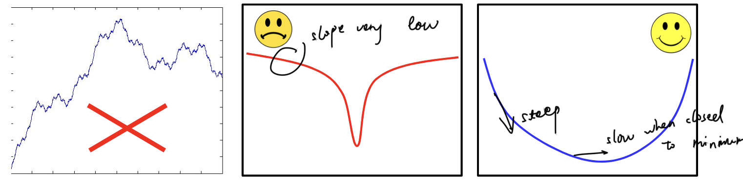
• What shape do we want the divergence function would be?
  • Must be smooth and not have many poor local optima
  • The best type of divergence is steep far from the optimum, but shallow at the optimum
    • But not too shallow(hard to converge to minimum)
• The choice of divergence affects both the learned network and results

• Common choices

  • L2 divergence

  $D i v=\frac{1}{2} \sum_{i}\left(y_{i}-d_{i}\right)^{2}$

  • KL divergence

    $D i v=\sum_{i} d_{i} \log \left(d_{i}\right)-\sum_{i} d_{i} \log \left(y_{i}\right)$

• L2 is particularly appropriate when attempting to perform regression

  • Numeric prediction
  • For L2 divergence the derivative w.r.t. the pre-activation of the output layer is :
    • $\nabla_{z} \frac{1}{2}\|y-d\|^{2}=(y-d) J_{y}(z)$
  • We literally “propagate” the error $(y-d)$ backward
  • Which is why the method is sometimes called “error backpropagation”

• The KL divergence is better when the intent is classification

  • The output is a probability vector

Batch normalization

• Covariate shifts problem

  • Training assumes the training data are all similarly distributed (So as mini-batch)
  • In practice, each minibatch may have a different distribution
  • Which may occur in each layer of the network
  • Minimize one batch cannot give the correction of other batches

• Solution

  • Move all batches to have a mean of 0 and unit standard deviation
  • Eliminates covariate shift between batches

• Batch normalization is a covariate adjustment unit that happens after the weighted addition of inputs (affine combination) but before the application of activation ⁵

• Steps

  • Covariate shift to standard position

  $u_{i}=\frac{z_{i}-\mu_{B}}{\sqrt{\sigma_{B}^{2}+\epsilon}}$

  • Shift to right position

    $\hat{z_i} = \gamma u_i + \beta$

Backpropagation

• The outputs are now functions of $\mu_B$ and $\sigma_B^2$ which are functions of the entire minibatch

$\operatorname{Div}(M B)=\frac{1}{B} \sum_{t} \operatorname{Div}\left(Y_{t}\left(X_{t}, \mu_{B}, \sigma_{B}^{2}\right), d_{t}\left(X_{t}\right)\right)$

• The divergence for each $Y_t$ depends on all the $X_t$ within the mini-batch
  • Is a vector function over the mini-batch
• Using influence diagram to caculate derivatives³

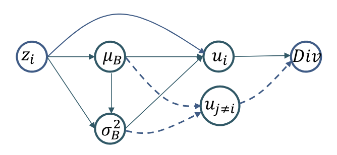
• Goal

  • We need to caculate the learnable parameters $\frac{d D i v}{\gamma}, \frac{d D i v}{\beta}$, and the affine combination $\frac{d D i v}{z_i}$

  $\frac{\partial D i v}{\partial z_{i}}=\frac{\partial D i v}{\partial u_{i}} \cdot \frac{\partial u_{i}}{\partial z_{i}}+\frac{\partial D i v}{\partial \sigma_{B}^{2}} \cdot \frac{\partial \sigma_{B}^{2}}{\partial z_{i}}+\frac{\partial D i v}{\partial \mu_{B}} \cdot \frac{\partial \mu_{B}}{\partial z_{i}}$

  • So we need extra $\frac{\partial D i v}{\partial u_{i}},\frac{\partial D i v}{\partial \sigma_{B}^{2}},\frac{\partial D i v}{\partial \mu_{B}}$

• Preparation

$\mu_{B}=\frac{1}{B} \sum_{i=1}^{B} z_{i}\quad \quad \sigma_{B}^{2}=\frac{1}{B} \sum_{i=1}^{B}\left(z_{i}-\mu_{B}\right)^{2}$

$u_{i}=\frac{z_{i}-\mu_{B}}{\sqrt{\sigma_{B}^{2}+\epsilon}} \quad \quad \hat{z_i} = \gamma u_i + \beta$

• For the first term $\frac{\partial D i v}{\partial u_{i}} \cdot \frac{\partial u_{i}}{\partial z_{i}}$

  • First caculate $\frac{d D i v}{\gamma}, \frac{d D i v}{\beta}$ $\frac{d D i v}{d \beta}=\frac{d D i v}{d \hat{z}} \quad \quad \frac{d D i v}{d \gamma}=u \frac{d D i v}{d \hat{z}}$

  • $\frac{\partial u_{i}}{\partial z_{i}} = \frac{1}{\sqrt{\sigma^2_B +\epsilon}}$, so the first term = $\frac{\partial D i v}{\partial u_{i}} \cdot \frac{1}{\sqrt{\sigma_{B}^{2}+\epsilon}}$

• For the second term $\frac{\partial D i v}{\partial \sigma_{B}^{2}} \cdot \frac{\partial \sigma_{B}^{2}}{\partial z_{i}}$

  • Caculate $\frac{\partial D i v}{\partial \sigma_{B}^{2}}$

  $\frac{\partial Div}{\partial \sigma_{B}^{2}}=\sum \frac{\partial Div}{\partial u_{i}} \frac{\partial u_{i}}{\partial \sigma_{B}^{2}}$

  $\frac{\partial D i v}{\partial \sigma_{B}^{2}}=\frac{-1}{2}\left(\sigma_{B}^{2}+\epsilon\right)^{-3 / 2} \sum_{i=1}^{B} \frac{\partial D i v}{\partial u_{i}}\left(z_{i}-\mu_{B}\right)$

  • And $\frac{\partial \sigma_{B}^{2}}{\partial z_{i}}$

  $\frac{\partial \sigma_{B}^{2}}{\partial z_{i}}=\frac{2\left(z_{i}-\mu_{B}\right)}{B}$

  • So the second term = $\frac{\partial D i v}{\partial \sigma_{B}^{2}} \cdot \frac{2\left(z_{i}-\mu_{B}\right)}{B}$

• Finally for the third term $\frac{\partial D i v}{\partial \mu_{B}} \cdot \frac{\partial \mu_{B}}{\partial z_{i}}$

  • Caculate $\frac{\partial D i v}{\partial \mu_{B}}$

  $\frac{\partial D i v}{\partial \mu_B}=\sum \frac{\partial Div}{\partial \mu_{i}} \frac{\partial \mu_{i}}{\partial \mu_{B}}+\frac{\partial Div}{\partial\sigma_{B}^{2} } \frac{\partial \sigma_{B}^{2}}{\partial \mu_{B}}$

  $\frac{\partial D i v}{\partial \mu_{B}}=\left(\sum_{i=1}^{B} \frac{\partial D i v}{\partial u_{i}} \cdot \frac{-1}{\sqrt{\sigma_{B}^{2}+\epsilon}}\right)+\frac{\partial D i v}{\partial \sigma_{B}^{2}} \cdot \frac{\sum_{i=1}^{B}-2\left(z_{i}-\mu_{B}\right)}{B}$

  • The last term is zero, and because $\mu_z = \frac{1}{B} \sum z_i$

  $\frac{\partial \mu_{B}}{\partial z_{i}}=\frac{1}{B}$

• So the third term = $\frac{\partial D i v}{\partial \mu_{B}} \cdot \frac{1}{B}$

• Overall

$\frac{\partial D i v}{\partial z_{i}}=\frac{\partial D i v}{\partial u_{i}} \cdot \frac{1}{\sqrt{\sigma_{B}^{2}+\epsilon}}+\frac{\partial D i v}{\partial \sigma_{B}^{2}} \cdot \frac{2\left(z_{i}-\mu_{B}\right)}{B}+\frac{\partial D i v}{\partial \mu_{B}} \cdot \frac{1}{B}$

$\frac{\partial D i v}{\partial \sigma_{B}^{2}}=\frac{-1}{2}\left(\sigma_{B}^{2}+\epsilon\right)^{-3 / 2} \sum_{i=1}^{B} \frac{\partial D i v}{\partial u_{i}}\left(z_{i}-\mu_{B}\right)$

$\frac{\partial D i v}{\partial \mu_{B}}=\frac{-1}{\sqrt{\sigma_{B}^{2}+\epsilon}}\sum_{i=1}^{B} \frac{\partial D i v}{\partial u_{i}}$

Inference

• On test data, BN requires $\mu_B$ and $\sigma_B^2$
• We will use the average over all training minibatches

$\mu_{B N}=\frac{1}{\text {Nbatches}} \sum_{b a t} \mu_{B}(\text {batch})$

$\sigma_{B N}^{2}=\frac{B}{(B-1) N b a t c h e s} \sum_{b a t c h} \sigma_{B}^{2}(\text {batch})$

• Note: these are neuron-specific
  • $\mu_B(batch), \sigma_B{batch}$ are obtained from the final converged network
  • The 𝐵/(𝐵 − 1) term gives us an unbiased estimator for the variance

What can it do

• Improves both convergence rate and neural network performance
  • Anecdotal evidence that BN eliminates the need for dropout
• To get maximum benefit from BN, learning rates must be increased and learning rate decay can be faster
  • Since the data generally remain in the high-gradient regions of the activations
  • e.g. For sigmoid function, move data to the linear part, the gradient is high
• Also needs better randomization of training data order

Smoothness

• Smoothness through network structure
  • MLPs are universal approximators
  • For a given number of parameters, deeper networks impose more smoothness than shallow&wide ones
  • Each layer restricts the shape of the function
• Smoothness through weight constrain

Regularizer

• The "desired” output is generally smooth
  • Capture statistical or average trends
• Overfitting
  • But an unconstrained model will model individual instances instead
  • Why overfitting?⁴
• Using a sigmoid activation, as $|w|$ increases, the response becomes steeper

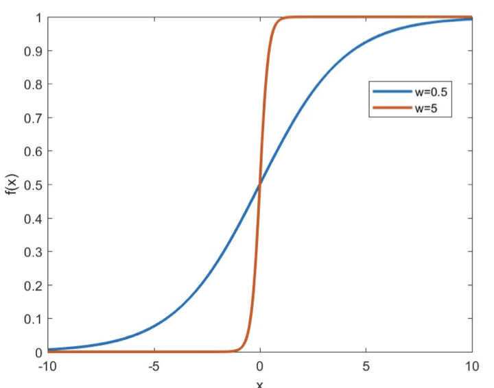
• Constraining the weights to be low will force slower perceptrons and smoother output response
• Regularized training: minimize the loss while also minimizing the weights

$L\left(W_{1}, W_{2}, \ldots, W_{K}\right)=\operatorname{Loss}\left(W_{1}, W_{2}, \ldots, W_{K}\right)+\frac{1}{2} \lambda \sum_{k}\left\|W_{k}\right\|_{2}^{2}$

• $\lambda$ is the regularization parameter whose value depends on how important it is for us to want to minimize the weights
• Increasing assigns greater importance to shrinking the weights
  • Make greater error on training data, to obtain a more acceptable network

Dropout

• “Dropout” is a stochastic data/model erasure method that sometimes forces the network to learn more robust models
• Bagging method
  • Using ensemble classifiers to improve prediction

• Dropout

  • For each input, at each iteration, “turn off” each neuron with a probability $1-\alpha$
  • Also turn off inputs similarly

• Backpropagation is effectively performed only over the remaining network

  • The effective network is different for different inputs
  • Effectively learns a network that averages over all possible networks (Bagging)

• Dropout as a mechanism to increase pattern density

  • Dropout forces the neurons to learn “rich” and redundant patterns
  • E.g. without dropout, a noncompressive layer may just “clone” its input to its output
  • Transferring the task of learning to the rest of the network upstream

Implementation

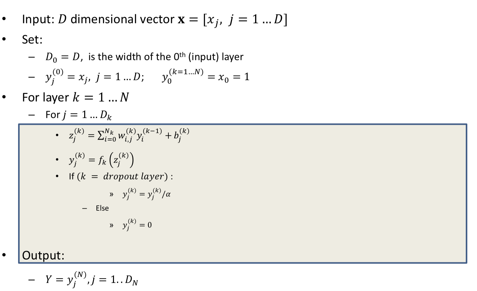
• The expected output of the neuron is $y_{i}^{(k)}=\alpha \sigma\left(\sum_{j} w_{j i}^{(k)} y_{j}^{(k-1)}+b_{i}^{(k)}\right)$

• During test, push the a to all outgoing weights

$\begin{aligned} z_{i}^{(k)} &=\sum_{j} w_{j i}^{(k)} y_{j}^{(k-1)}+b_{i}^{(k)} \\\\ &=\sum_{j} w_{j i}^{(k)} \alpha \sigma\left(z_{j}^{(k-1)}\right)+b_{i}^{(k)} \\\\ &=\sum_{j}\left(\alpha w_{j i}^{(k)}\right) \sigma\left(z_{j}^{(k-1)}\right)+b_{i}^{(k)} \end{aligned}$

• So $W_{test} = \alpha W_{trained}$
  • Instead of multiplying every output by all weights by $\alpha$, multiply all weight by $\alpha$
• Alternate implementation
  • During training, replace the activation of all neurons in the network by $\alpha ^{-1} \sigma(.)$
  • Use $\sigma(.)$ as the activation during testing, and not modify the weights

More tricks

• Obtain training data
  • Use appropriate representation for inputs and outputs
  • Data Augmentation
• Choose network architecture
  • More neurons need more data
  • Deep is better, but harder to train
• Choose the appropriate divergence function
  • Choose regularization
• Choose heuristics
  • batch norm, dropout ...
• Choose optimization algorithm
  • Adagrad / Adam / SGD
• Perform a grid search for hyper parameters (learning rate, regularization parameter, …) on held-out data
• Train
  • Evaluate periodically on validation data, for early stopping if required

¹. A good summary of recent optimizers can be seen in here. ↩

². Animations for optimization algorithms ↩

³. A simple and clear demostration of 2 variables in a single network ↩

⁴. The perceptrons in the network are individually capable of sharp changes in output ↩

⁵. Batch normalization in Neural Networks ↩